Risk Quantification in Mega-Infrastructure Project Portfolios

Mega-infrastructure project portfolios—spanning utility smart grid retrofits, regional fiber rollouts, and trans-continental transportation lines—are characterized by high capital commitments, multi-year delivery timelines, and massive systemic uncertainty. Traditional deterministic planning assumes single-point schedule and cost estimates, leading to structural optimism bias and systematic cost overruns. To protect capital investments, portfolio managers utilize quantitative risk analysis. By integrating Expected Monetary Value (EMV), Decision Tree models, and Monte Carlo probability simulations, organizations can model portfolio uncertainty scientifically, establishing realistic contingency reserves and joint confidence boundaries. This guide outlines the mathematical foundation and governance frameworks for quantitative risk management.

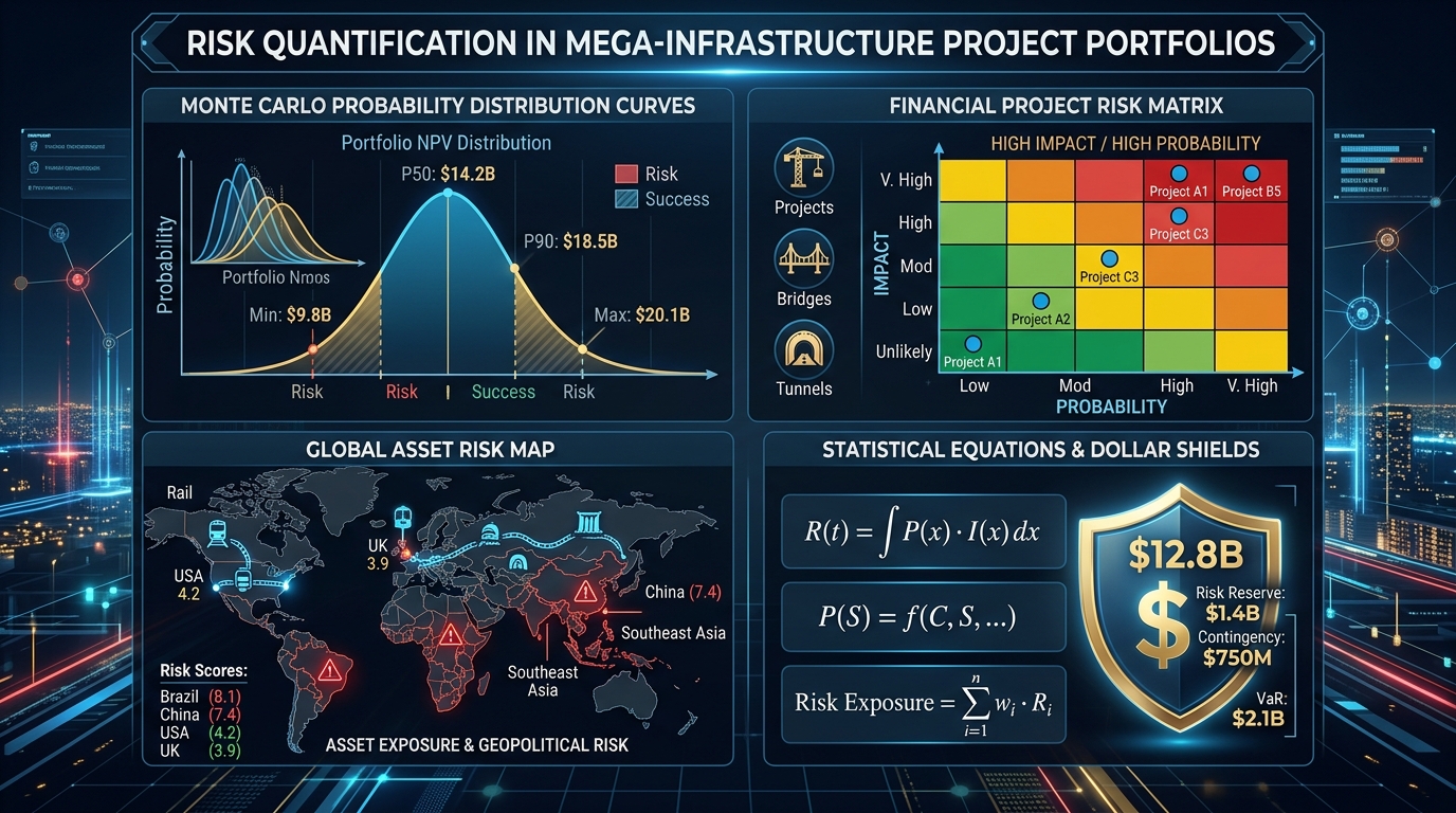
Figure 1: Monte Carlo probability S-curve showing cost contingency allocation at different confidence levels.

1. The Flaw of Deterministic Estimation in Mega-Projects

Mega-projects systematically fail to meet cost and schedule baselines due to complex, compounding risk dependencies. Deterministic planning is structurally flawed: it assumes every activity completes exactly on its target date. However, in the real world, project execution is subject to non-deterministic variables: delayed environmental permits, labor disputes, material cost inflation, and weather disruptions. When these risks interact, they create non-linear compounding delays. For instance, a 2-week delay in substation foundation pouring can miss a dry weather window, pushing subsequent electrical installations into a 3-month winter freeze period. Quantitative risk analysis replaces deterministic single-point values with range estimates represented by probability distribution functions, allowing portfolio managers to calculate the probability of achieving specific project targets and establish risk-adjusted baselines from the outset.

2. Expected Monetary Value (EMV) & Decision Tree Formulations

The first step in quantitative risk analysis is evaluating discrete risk events using Expected Monetary Value (EMV). EMV calculates the statistical average of future uncertain outcomes by multiplying the probability of occurrence by the financial impact of the event: EMV = Probability * Impact. By calculating EMV across the portfolio risk register, project managers can prioritize risks objectively based on their financial exposure rather than subjective scoring. Furthermore, decision tree analysis models sequential decision pathways, mapping alternate choices, event branches, and terminal values. Portfolio managers calculate the EMV of each decision path, identifying the optimal strategic direction that minimizes risk exposure and maximizes return on investment.

3. Monte Carlo Simulations for Schedule & Cost S-Curves

While EMV analyzes discrete risk events, Monte Carlo simulation models the cumulative impact of all project uncertainties simultaneously. Monte Carlo analysis executes thousands of computer-generated project iterations, randomly sampling activity durations and cost variations from predefined probability distribution functions to generate cumulative probability curves (S-curves). These S-curves show the probability of completing the project within specific schedule dates and budget boundaries. For example, a Monte Carlo simulation may reveal that while the target schedule date indicates a June 1 completion, there is only a 15% probability (P15) of achieving that target. By evaluating the S-curve, the portfolio manager can establish a P80 baseline (80% probability of completion), ensuring that schedule commitments to external stakeholders are statistically viable.

4. Choosing the Right Probability Distribution Functions

Accurate Monte Carlo modeling requires selecting the appropriate probability distribution function (PDF) for each activity duration and cost package: Triangular Distribution: Defined by three values: Minimum, Most Likely, and Maximum. Used when historical data is limited but expert opinion can define boundary constraints. Beta (PERT) Distribution: Similar to triangular but places heavier weight on the most likely value, producing a smoother probability curve that fits traditional engineering activities. Lognormal Distribution: Characterized by a long right-hand tail, representing activities that cannot finish early but suffer severe unbounded delays (e.g. regulatory approvals or environmental litigation). Normal (Gaussian) Distribution: Symmetric distribution used for highly standardized, repetitive tasks with predictable variation (e.g. fiber splicing or meter installations).

5. Quantitative Risk Breakdown Structures (RBS)

Portfolio managers utilize Risk Breakdown Structures (RBS) to organize and categorize risks across the entire organization. The RBS decomposes risk into hierarchy tiers: Technical (compatibility, complexity, performance), External (regulatory, permitting, weather), Organizational (resourcing, funding, priorities), and Project Management (estimation, control, communication). Integrating the RBS with the Work Breakdown Structure (WBS) creates a Risk-WBS matrix, linking specific risk events directly to individual work packages. This mapping ensures that risk owners are assigned to every high-impact package and that cost contingency reserves are allocated directly to the WBS nodes where the risk resides.

6. Sensitivity Analysis & Tornado Diagram Interpretation

Sensitivity analysis identifies which specific risks have the greatest impact on the project timeline or budget. The results of sensitivity analysis are plotted on a Tornado Diagram, a bar chart where horizontal bars are ordered by impact magnitude. The widest bars at the top represent the critical risks driving portfolio variance (e.g. substation transformer shipping delays). The narrow bars at the bottom represent minor risks that have negligible impact. By reviewing the Tornado Diagram, portfolio managers can focus executive attention and mitigation budgets on the top three risk drivers, optimizing risk response spending and maximizing schedule protection.

7. Contingency Buffer Allocation & Management Reserves

To secure portfolio delivery, organizations calculate Joint Confidence Levels (JCL). A JCL integrates cost and schedule S-curves, calculating the probability that the project will complete both on time AND under budget. To achieve a JCL of 80% (P80 for both cost and schedule), managers allocate specific Schedule Buffers and Cost Contingency Reserves. Cost contingency is calculated using Monte Carlo output variance at the P80 confidence level and held in a centralized management reserve pool. Schedule buffers are placed immediately preceding major project integration gates rather than scattered across individual activities, preventing Parkinson’s Law (work expanding to fill available time) from eroding the buffer.

8. Risk Response Execution Strategies

Once risks are quantified, portfolio managers execute formal risk response strategies defined by the PMI framework: Avoid: Eliminate the risk by changing the project plan (e.g., re-routing a fiber backbone to avoid a disputed geographical zone). Mitigate: Reduce the probability or impact of the risk (e.g., conducting early soil testing to prevent structural foundation design changes). Transfer: Shift the financial impact of the risk to a third party (e.g., purchasing performance bonds or structuring contracts as fixed-price turnkey). Accept: Acknowledge the risk and establish contingency reserves to absorb the impact if the event occurs.

9. Quantitative Risk Audit: Substation Modernization Case Study

A major regional utility modernizing 45 substations deployed this quantitative risk model. The initial deterministic schedule projected completion in 18 months under a $50M budget. However, Monte Carlo simulation revealed a JCL of only 12% for these targets. The simulation identified environmental permitting and vendor transformer delivery delays as the primary variance drivers. By allocating a 3-month centralized schedule buffer and a $4.2M contingency reserve (achieving a verified JCL of 80%), and transferring transformer shipping risks via contractual SLA clauses, the utility successfully completed the program in 21 months within the revised $54.2M budget, avoiding costly emergency funding requests.

10. Enterprise Risk Governance & Software Tooling

Maintaining quantitative risk alignment requires deploying enterprise risk management software (such as Primavera Risk Analysis, @RISK, or Safran Risk). These tools integrate directly with scheduling databases, allowing risk managers to update probability distributions weekly. Executive dashboards present risk metrics using simplified KPIs, showing current contingency consumption rates against project progress, and alerting the C-suite when risk drawdown speeds indicate emerging systemic distress.

11. Real Options Valuation & Strategic Project Flexibility

In mega-projects with long execution horizons, traditional Discounted Cash Flow (DCF) metrics like Net Present Value (NPV) fail to capture the value of managerial flexibility to adapt to changing market conditions. Portfolio managers apply Real Options Valuation (ROV) to value strategic choices as financial options.

Under ROV, managers evaluate options to defer (waiting to invest until regulatory uncertainty resolves), option to expand (scaling a fiber network rollout to adjacent cities if demand exceeds initial targets), or option to abandon (terminating a project early to limit capital loss if pilot results fail). Integrating real options into the risk quantification framework provides a mathematically rigorous approach to valuing strategic agility.

12. Executive Summary & Portfolio Risk Governance Checklist

In summary, quantitative risk management transforms portfolio governance from a subjective, reactive process into a predictive, data-driven science. By defining range estimates, running Monte Carlo simulations, and calculating Joint Confidence Levels, organizations secure capital investments and ensure mega-project delivery success.

Establishing dedicated risk ownership, conducting sensitivity analyses to focus resources on top drivers, and deploying modern probabilistic scheduling software protects public and private investments from severe optimism bias and ensures predictable capital allocation.

Academic & Industry References

1. Project Management Institute. (2021). A Guide to the Project Management Body of Knowledge (PMBOK Guide) – Seventh Edition. PMI.
2. Flyvbjerg, B. (2014). What You Should Know About Megaprojects and Why: An Overview. Project Management Journal.
3. Kerzner, H. (2017). Project Management: A Systems Approach to Planning, Scheduling, and Controlling (12th ed.). John Wiley & Sons.